A Novel Colour Gradients Based CFA Interpolation Algorithm

Roop Kumar V
Department of Electronics and Communication Engineering,QIS College of Engineering & Technology,Ongole, Andhra Pradesh, India.
email: vadderoopkumar@yahoo.com

----------------------------------------------------------------------------------------------------------------------------------------------------------------------------------------------------------------------------------------------------------------------------

ABSTRACT

The primary colour components (Green, Red, and Blue) are captured through single-sensor digital colour cameras mounted with a colour filter array (CFA) at all pixel locations through CFA. The limitations of the sensors used in the commercial digital cameras make the camera to capture only a sub-sampled image where each pixel contains only partial colour information. Consequently, the estimation of missing colour samples is Critical to Reconstruct the full colour picture. The process of Calculating the missing colour samples is known as demosaicking. The demosaicking is a critical step, in producing a high-quality colour image. Among Numerous demosaicking methods, directional filtering-based methods found to be most efficient. These techniques utilize the inherent directional colour gradients in the image to guide the interpolation process, thus preserving edges and reducing artifacts. In this research work, a simple yet effective approach is proposed to demosaicking that leverages the principles of directional filtering. By optimizing the balance between simplicity and efficiency, our proposed method provides high-quality colour image reconstruction making it appropriate for applications and devices with less power at their disposal for processing.

Keywords:

Colour filter array, Colour gradients, Demosaicking, Directional filtering, Estimation, Interpolation, Primary Colour Components, Processing power, Single Sensor Digital Colour Cameras, Sub-sampled.

1. INTRODUCTION

Each individual sensor [1] can capture only one colour of the Image through the Colour Filter Array [2] mounted on a Single CCD/CMOS sensor [3] commercial Digital Colour Camera [4]. To reconstruct a full-colour (RGB) image [5], both luminance and chrominance information must be sampled. The human visual system (HVS) [6] is more sensitive to changes in luminance information than to degradations in chrominance information. Consequently, chrominance channels are often sub-sampled more heavily than luminance channels. In other words, chrominance channels may be sampled at a significantly lesser rate than luminance channels due to this required sub-sampling. The spectral sensitivity of the HVS to luminance [7] exhibits a strong correlation with the spectral power distribution of the green channel, whereas the R and B channels are more closely associated with the chrominance components. Therefore, green sensors serve as the luminance channel, while red and blue sensors serve as the chrominance channels.

The Bayer [8] array [9], as shown in the Figure 1, is extensively used. In this array, green filters are arranged in a quincunx configuration, while the red and blue filters are allocated to the remaining spatial positions. The pattern is repeated both horizontally and vertically across the entire sensor array, covering both spatial dimensions.

Figure 1: Possible Bayer Colour Filter Arrays

The CFA is positioned between the lens and the sensor array generates a 'mosaic' of colour samples [10]. This mosaic [11] processed to reconstruct three full colour planes, is called as demosaicking [12], involves estimating or interpolating [13] techniques. Various methods for this interpolation process will be discussed. The structure of the remaining work is ordered as follows. The Section II provides the methodology of the "Algorithm for CFA Interpolation based on Colour Gradients”. Section III provides the quality evaluation, and Section IV presents the concluding remarks and future work, followed by references and an appendix for detailed results.

Demosaicking methods can generally be categorized into three main groups: interpolation-based methods [14], [15], [16], [17], [18], Optimization-based methods [19], [20], [21], [22] and learning- based methods [23], [24], [25], [26], [27]. Interpolation-based methodologies, despite their widespread application, often induce the deterioration of edge information and the attenuation of textural details, ultimately impeding the accurate reconstruction of essential structural features within the image. In contrast, optimization-based frameworks characterize demosaicking as an ill-posed inverse problem, wherein the solution is not uniquely determined and is sensitive to perturbations in the input data. These approaches capitalize on inter-channel dependencies within color-difference domains or utilize sparse coding techniques to model image patches, thereby enhancing the fidelity of the reconstructed images. Although these methods have seen some improvements, they frequently struggle with areas of strong texture, leading to the introduction of undesirable visual artifacts due to hard coding and reliance on manual heuristics.

2. METHODOLOGY

The performance evaluation of demosaicking algorithms is crucial in determining the overall performance of a digital camera. Over time many demosaicking algorithms are designed and developed. The fundamental questions for any engineer looking to design a new demosaicking algorithm or select an existing one is identifying the Problem and difference between implementation and performance. In an attempt to address some of these questions, this work investigates several noteworthy demosaicking algorithms, including Edge Sensing Interpolation Algorithm, Bilinear Interpolation, Alternating Projections, and High-Quality Linear Interpolation.

Algorithm for CFA Interpolation based on Colour Gradients:

This demosaicking algorithm is grounded in colour gradient estimation using directional filtering, applied to reconstruct the high-fidelity green channel. Subsequently, the red and blue channels are interpolated by utilizing the spatial information embedded within the green channel. An advanced approach involves generating two complete colour images through independent interpolation along the horizontal and vertical axes, thereby optimizing the reconstruction process. In this algorithm, a similarity metric is computed by estimating the horizontal and vertical gradient components.

Algorithm:

Step1: Obtain CFA Data
Step2: Perform Horizontal& Vertical Interpolations on Green Channel.
Step3: Fully populate green channel by judiciously estimating the green pixel from the above Two interpolated green channels.
Step4; Interpolate Red and Blue Channels using the result obtained in Step3. Step5: Combine the R, G, B channels to get the full Colour image.
Step6: Compare the obtained results with those of state-of-the-art algorithms and provide an analysis of the findings.

The algorithm commences by reconstructing the green channel along both horizontal and vertical axes. To perform interpolation of the Bayer samples, a five-tap finite impulse response (FIR) filter is utilized, optimizing the spatial reconstruction process. The use of a longer filter is deliberately avoided to mitigate the occurrence of zipper artifacts near edges, as noted in [28] [29] [30]. The filter applied is identical to that described in [31] [32], and its coefficients are determined based on specific considerations. It is important to observe that the green signal in the Bayer pattern is subsampled by a factor of 2 along each row or column. The frequency domain representation is given as,

Here, G(ω) and G_s(ω) represent the Fourier Transforms of the original green signal and the down-sampled green signal, respectively. If we interpolate it with the band-limited filter, we have

The second term in the equation signifies the aliasing component. To mitigate aliasing-induced distortions and enhance the mid-frequency spectral response, an optimal approach entails incorporating data from the high-frequency spectral bands of the red and blue channels, exploiting the well-established inter-channel correlations in their high-frequency components. Within the context of a green-red row, the red channel is spatially sampled with a one-sample offset relative to the green channel signal, thereby optimizing spatial alignment and facilitating precise interpolation. Consequently, its Fourier transform yields

Here, R(ω) represents the Fourier Transform of the original red signal. If we interpolate it with a filter h1 and we add the resulting signal to Equation (3) is

Here, R(ω) denotes the Fourier Transform of the original red signal. If this signal is interpolated using a filter h1h_1h1, the resulting signal is subsequently added to Equation (3), yielding:

Reminding us that R(ω)-G(ω) is slowly varying, if h₁ is designed such that H₁(ω) at low frequencies and H₁(ω)≅ H₀(ω) at high frequencies, we have

and

and Equation (4), could be approximated as

A right choice for the filter h1 that respects the constraints in Equation (5) and (6) is the five-coefficient FIR filter is represented as [-0.25 0 0.5 0 -0.25]

Therefore, in the following row of the Bayer-sampled image:

. . . 𝑅₂ 𝐺₁ 𝑅₀ 𝐺₁ 𝑅₂ . . .

the green sample G0 is estimated as

An interesting interpretation of Equation (8) is supplied by Wu and Zhang in [30], where they note that (8) can be written as

The interpolation of green values within the blue-green rows and along the columnar axis is executed through a unified computational paradigm. After performing interpolation of the green component in both horizontal and vertical orientations—yielding two distinct reconstructions of the green channel—a selection must be made to identify the filtering direction that maximizes reconstruction accuracy. Upon finalizing the reconstruction of the green channel, the red and blue components are subsequently interpolated to attain complete spectral reconstruction. In addition to the Bayer data, the reconstructed full-resolution green image, denoted as 𝐺̂, is now available and can be utilized for reconstructing the remaining two components.

The prevailing technique for estimating the red and blue components involves interpolating the color differences, R−G and B−G, rather than directly interpolating the R and B channels. Nonetheless, bilinear interpolation remains the most adopted method, frequently modified for the reconstruction of the red (or blue) component at the blue (or red) pixel locations. In such instances, edge-directed interpolation is employed to interpolate the color differences along one of the two diagonal orientations, exploiting local edge information and image gradient distributions to optimize the accuracy of the reconstruction process.

3. EXPERIMENTAL RESULTS

Reconstruction accuracy and Performance evaluation of a demosaicking algorithms can be evaluated from two perspectives: Objective Evaluation and subjective Evaluation. There are numerous metrics used in literature to determine the accuracy of the reconstruction, such as Mean Square Error (MSE), Peak Signal to Noise Ratio (PSNR) [32]The error between the two images is defined as

and the MSE between 𝑓(𝑚, 𝑛) and 𝑓(𝑚, 𝑛) is the square root of the error square averaged over the 𝑀 × 𝑁 array, or

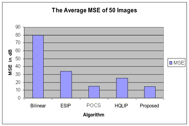
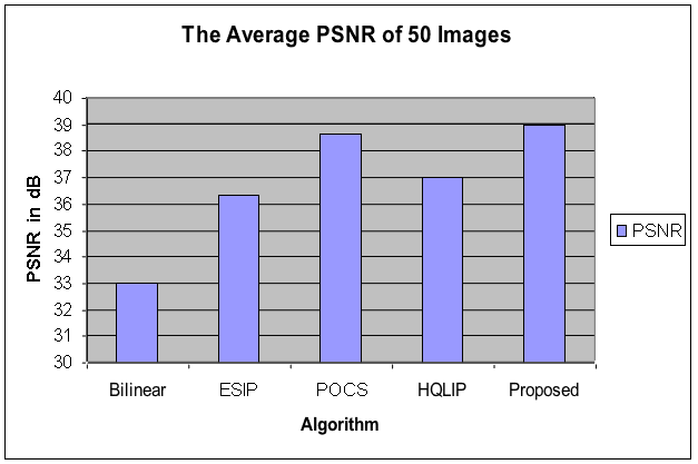
The Average mean square error of the tested algorithms on the 50 datasets is given in results. PSNR in dB is defined as

1. Experiment Setup:

• Experiments conducted using a dataset of 50 images, with dimensions of 512×512 pixels and 3 colour channels (RGB).
• These dataset images sampled corresponding to the Bayer pattern. This pattern is commonly used in digital camera sensors to capture colour information by alternating rows of R-G and B-G pixels.
• Different demosaicking techniques were applied to reconstruct the images from sub-sampled images along with the proposed algorithm.

2. Evaluation Metrics:

• Mean Squared Error (MSE) and Peak Signal-to-Noise Ratio (PSNR) are commonly utilized metrics for assessing the performance of demosaicking algorithms.
• MSE quantifies the average squared deviation between the original and restored pixel intensities.
• PSNR quantifies the ratio between the maximal theoretical signal power and the power of the noise that impairs the accuracy and fidelity of its reconstruction.

3. Results Summary:

• The results of the experiments are tabulated in Table-1.
• The proposed algorithm exhibits superior performance compared to all other methods, as evidenced by its reduced mean squared error (MSE) and enhanced peak signal-to-noise ratio (PSNR), indicating a higher level of fidelity in the reconstructed images. This indicates that the reconstructed images using the proposed algorithm have lower error and higher fidelity compared to the others.

4. Detailed Results:

• More detailed results, presumably including individual performance metrics for each algorithm tested, are available in the appendix. These results provide a deeper insight into the performance of each technique.

Figure 2: Test Dataset

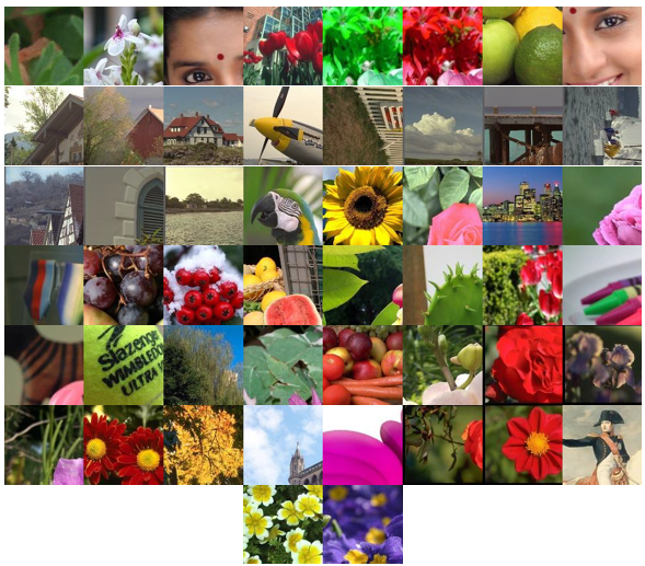
Table 1: Mean Square Error of 50 sets of Images

Img	Bilinear			ESIP			POCS			HQLIP			Proposed
	R	G	B	R	G	B	R	G	B	R	G	B	R	G	B
1	161	88	173	40	47	44	8.4	5.5	17	29	28	37	11	7.4	13
2	222	107	196	68	61	74	16	6.8	19	71	22	71	11	8	13
3	9	5.8	8.9	2.3	1.7	2.5	1.3	1	2.9	1.6	2.1	4	1.6	0.8	2
4	446	164	461	78	67	86	21	9	25	148	34	130	18	11	20
5	167	76	158	48	47	52	9.2	5.2	15	46	18	51	12	7.9	16
6	106	46	94	29	26	28	6.6	4.6	8	28	12	28	11	5.2	8
7	11	6.2	9.1	4.2	3.9	5	1.5	0.8	2.3	3	1.9	5.3	1.9	1	2.3
8	129	65	135	29	26	32	8.4	4.3	12	38	17	44	9.6	6.1	11
9	123	61	105	30	31	34	7.9	5.1	20	32	15	42	10	6.2	13
10	181	84	179	43	39	45	11	5.9	14	55	20	57	14	9	16
11	71	41	74	35	34	37	8.1	6	13	22	11	25	12	8.6	14
12	81	48	94	33	36	36	6.3	3.4	9.8	24	11	28	7.6	6.4	10
13	1.1	0.5	1.1	0.6	0.3	0.6	0.6	0.3	0.6	0.6	0.3	0.7	0.6	0.2	0.6
14	15	7.6	20	5	3.7	7.1	2.8	1.6	5.4	3.8	3.2	6.4	2.8	1.6	5.2
15	13	5.8	13	13	3.8	8	19	8.6	12	10	4.8	9.2	19	5.4	12
16	12	5.3	11	6.5	3.8	6.4	7.7	5.4	7.2	4.2	3.5	5.1	8.7	4.1	8
17	105	39	106	20	14	17	17	8	8.9	37	12	35	14	4.8	7.1
18	4.1	2	3.4	1.2	0.7	1	0.9	0.5	0.8	1	0.8	1.1	0.9	0.4	0.9
19	55	31	81	22	17	36	24	23	48	19	16	31	18	11	38
20	2.4	0.9	2.2	4.4	0.9	3.7	7.4	4.7	6	3.2	2	3.7	6.5	2.9	5.3
21	24	11	27	9.5	7.5	18	10	8.3	22	9.8	6.4	17	9.7	5.7	21
22	163	77	153	41	44	40	15	9.1	20	40	20	32	15	10	22
23	134	57	121	47	42	48	16	7.3	14	42	21	40	21	12	18
24	91	54	53	36	41	37	33	30	30	36	18	31	35	24	34
25	12	5.2	11	4.1	2.6	3.4	4.6	2.4	2.8	3.5	2.5	3.5	4.2	1.5	2.8
26	10	7.6	14	9	4.3	8.2	11	7	9.1	6.1	3.5	7.8	8.9	3.3	7.5
27	81	36	77	26	22	24	9.5	4.5	8.9	26	11	24	10	5.1	9
28	474	252	373	170	188	167	71	58	78	147	67	106	86	63	87
29	99	53	64	39	35	35	41	25	26	36	15	26	37	17	28
30	18	7.8	18	4	2.8	4.9	2.9	2.1	4.1	5.5	3.2	5.5	2.7	1.4	3.5
31	47	23	48	15	14	15	5.1	2.5	4.8	13	7.1	12	6.5	3.7	6.7
32	29	9.8	23	11	8.1	7.6	15	5	5	10	5.8	8.2	14	3.9	5.3
33	93	44	94	17	20	18	4.6	3	7.2	22	10	18	4.5	3.4	6.3
34	18	8	19	9.8	4.7	8.5	12	4.9	8.5	8.9	3.9	9.1	9.5	3	7.2
35	12	4.1	11	9.3	2.5	7	14	7.8	9.9	6.7	5.3	7.3	12	4.2	8.9
36	144	64	150	60	50	60	16	7.5	17	45	17	39	15	10	17
37	119	63	119	55	47	66	21	16	35	40	16	47	22	15	38
38	3.3	0.7	2.1	2.6	0.5	1.8	3.9	1.5	2.6	2.8	1	2.2	3.6	0.9	2.4
39	6.2	2.1	4.1	8.5	1.7	5.2	9.8	4.5	5.6	5.8	2.5	4.6	10	2.4	5.9
40	16	6.3	18	15	4.1	10	20	11	15	10	7	11	21	6.8	15
41	20	9	23	6.6	6.1	7.5	2.9	2.1	4.7	5.7	3.8	5.3	3.3	2.2	4.9
42	38	22	28	14	15	16	13	8.5	14	9.6	7.6	15	11	4	13
43	103	54	115	41	26	35	36	20	29	42	18	42	30	11	22
44	51	27	61	58	19	25	85	30	39	41	15	30	70	16	30
45	39	18	35	19	13	15	14	5.7	8.4	13	6.1	12	14	5	9
46	3.2	1	4.6	3.2	0.8	4.2	5.4	2.9	6.5	3.1	1.7	4.7	4	1.3	5.1
47	54	33	64	24	28	26	13	11	14	19	13	18	14	9.4	13
48	606	299	594	255	217	263	96	45	100	230	76	198	95	59	109
49	29	22	38	21	18	20	19	12	17	15	11	18	16	7.8	15
50	498	260	310	238	220	173	90	67	69	193	61	97	91	66	87
Avg	98.986	48.294	91.930	35.616	31.370	34.492	17.896	10.626	17.480	33.278	13.820	30.114	17.722	9.720	17.378
Avg RGB	79.737			33.826			15.334			25.737			14.940

Table 1: Mean Square Error of 50 sets of Images

Table 2 — Peak Signal to Noise Ratio of 50 Sets of Images

Img	Bilinear (R G B)			ESIP (R G B)			POCS (R G B)			HQLIP (R G B)			Proposed (R G B)
	R	G	B	R	G	B	R	G	B	R	G	B	R	G	B
1	26	29	26	32	31	32	39	41	36	33	34	32	38	39	37
2	25	28	25	30	30	29	36	40	35	30	35	30	38	39	37
3	39	40	39	45	46	44	47	48	44	46	45	42	46	49	45
4	22	26	21	29	30	29	35	39	34	26	33	27	36	38	35
5	26	29	26	31	31	31	38	41	36	32	36	31	37	39	36
6	28	32	28	33	34	34	40	42	39	34	37	34	38	41	39
7	38	40	39	42	42	41	46	49	45	43	45	41	45	48	44
8	27	30	27	34	34	33	39	42	37	32	36	32	38	40	38
9	27	30	28	33	33	33	39	41	35	33	36	32	38	40	37
10	26	29	26	32	32	32	38	40	37	31	35	31	37	39	36
11	30	32	29	33	33	32	39	40	37	35	38	34	37	39	37
12	29	31	28	33	33	33	40	43	38	34	38	34	39	40	38
13	48	52	48	50	53	50	50	53	50	51	53	50	50	54	51
14	36	39	35	41	42	40	44	46	41	42	43	40	44	46	41
15	37	40	37	37	42	39	35	39	37	38	41	39	35	41	37
16	38	41	38	40	42	40	39	41	40	42	43	41	39	42	39
17	28	32	28	35	37	36	36	39	39	32	37	33	37	41	40
18	42	45	43	47	50	48	49	51	49	48	49	48	48	52	49
19	31	33	29	35	36	33	34	35	31	35	36	33	36	38	32
20	44	49	45	42	49	42	39	41	40	43	45	42	40	44	41
21	34	38	34	38	39	35	38	39	35	38	40	36	38	41	35
22	26	29	26	32	32	32	36	39	35	32	35	33	36	38	35
23	27	31	27	31	32	31	36	40	37	32	35	32	35	37	36
24	29	31	31	33	32	32	33	33	33	33	35	33	33	34	33
25	37	41	38	42	44	43	42	44	44	43	44	43	42	46	44
26	38	39	37	39	42	39	38	40	39	40	43	39	39	43	39
27	29	33	29	34	35	34	38	42	39	34	38	34	38	41	39
28	21	24	22	26	25	26	30	31	29	26	30	28	29	30	29
29	28	31	30	32	33	33	32	34	34	32	36	34	32	36	34
30	35	39	36	42	44	43	28	31	28	32	34	33	36	39	36
31	31	34	31	36	37	36	41	44	41	37	40	37	40	42	40
32	32	33	38	34	38	39	39	36	41	41	38	40	39	37	42
33	41	33	28	32	28	36	35	36	41	43	40	34	36	39	35
34	38	41	39	37	40	37	37	41	39	37	40	37	37	41	39
35	46	43	48	42	43	49	42	41	43	40	43	46	41	42	47
36	31	33	30	34	34	34	37	38	37	35	37	36	37	38	37
37	38	42	37	43	44	43	42	46	44	41	44	41	43	47	41
38	20	23	20	24	25	24	28	32	28	25	29	25	28	30	28
39	33	35	32	35	36	35	35	37	36	36	38	36	36	39	36
40	21	24	23	24	25	26	29	30	30	25	30	28	29	30	29
41	31	33	30	34	34	34	37	38	37	35	37	36	37	38	37
42	38	41	39	37	40	37	36	41	39	37	40	37	37	41	39
43	50	45	44	51	46	42	46	44	44	48	45	43	48	44	37
44	39	40	45	42	39	46	41	38	42	41	40	44	41	38	35
45	40	36	40	39	37	42	38	38	44	40	35	37	42	38	33
46	44	45	41	41	42	41	43	45	41	42	45	41	43	46	41
47	32	35	34	37	36	36	37	39	37	38	39	36	38	42	37
48	20	23	20	24	25	24	28	32	28	25	29	25	28	30	28
49	33	35	32	35	36	35	35	37	36	36	38	36	36	39	36
50	21	24	23	24	25	26	29	30	30	25	30	28	29	30	29
Avg	32	35	32	36	37	36	38	40	38	36	39	36	38	41	38
Avg RGB	33			36.33			38.66			37			39

Table 2: Peak Signal to Noise Ratio of 50 sets of Images

Figure 3: The Average MSE of 50 Images
Figure 4: The Average PSNR of 50 Images

Method	Channel	MSE		PSNR
		Avg	Avg RGB	Avg	Avg RGB
Bilinear [33]	RED	99	79.66	32	33
	GREEN	48		35
	BLUE	92		32
ESIP [34] [35]	RED	36	34	36	36.33
	GREEN	31		37
	BLUE	35		36
POCS [36]	RED	18	15.33	38	38.66
	GREEN	11		40
	BLUE	17		38
HQLIP [37]	RED	33	25.66	36	37
	GREEN	14		39
	BLUE	30		36
Proposed	RED	18	14.93	38	39
	GREEN	9.8		41
	BLUE	17		38

Table 3: The Average MSE and PSNR of 50 Images

The table compares the performance of several demosaicking algorithms (Bilinear, ESIP, POCS, HQLIP, and a proposed algorithm) based on Mean Squared Error (MSE) and Peak Signal-to-Noise Ratio (PSNR) across R, G and B color channels. The data represents the average results across 50 images

The summary of the key findings:

MSE (Lower is better): The proposed algorithm consistently achieves the lowest MSE values across all color channels (Red: 18, Green: 9.8, Blue: 17). POCS is a close second, with similar MSE values. Bilinear performs significantly worse, with much higher MSE values. PSNR (Higher is better): Correspondingly, the proposed algorithm and POCS achieve the highest PSNR values. The proposed algorithm shows a slightly better PSNR for Green (41) and very similar for Red and Blue (38 and 38 respectively) compared to POCS. Bilinear has the lowest PSNR values. Overall Performance: The proposed algorithm and POCS demonstrate superior performance compared to the other algorithms in terms of both MSE and PSNR. The proposed algorithm edges out POCS slightly in PSNR for the Green channel and has a slightly lower MSE for Green as well. Bilinear is clearly the least effective of the methods tested.

In simpler terms, the proposed demosaicking algorithm produces reconstructed images with the least amount of error (low MSE) and the highest quality (high PSNR) compared to the other algorithms tested. This substantiates the assertion made in the introductory section that the proposed algorithm surpasses the other methods in terms of both MSE and PSNR.

4. CONCLUSION AND FUTURE WORK

This study meticulously evaluated the performance of various demosaicking algorithms, including Bilinear, ESIP, POCS, HQLIP, and a newly proposed methodology, employing objective evaluation metrics such as MSE and PSNR. The results, based on an extensive aggregate analysis of 50 images, unequivocally establish the superior efficacy of the proposed algorithm in comparison to the alternatives. It consistently exhibited the lowest MSE values across all color channels (R, G, and B), indicating a negligible discrepancy between the reconstructed and original images, thereby highlighting its efficacy in preserving image fidelity. Consequently, the proposed algorithm also yielded the highest PSNR values, signifying higher image quality with less noise and distortion. While the POCS algorithm showed competitive performance, particularly in MSE, the proposed algorithm consistently matched or slightly exceeded its PSNR performance, especially in the green channel. The Bilinear interpolation method proved to be the least effective, exhibiting significantly higher MSE and lower PSNR values compared to the other algorithms. These findings confirm the efficiency of the proposed demosaicking approach in generating high-quality color images from Bayer pattern data.

Future Work:

While the proposed algorithm demonstrates promising results, several avenues for future research can be explored:

• Computational Complexity Analysis: This study focused on image quality metrics. Future work could investigate the computational complexity and processing time of the proposed algorithm compared to other methods. This analysis is crucial for real-time applications and resource-constrained devices.
• Testing on Diverse Image Datasets: The evaluation was based on a set of 50 images. Expanding the testing to include a more diverse and larger dataset, encompassing various image types (e.g., natural scenes, textures, portraits), would provide a more comprehensive assessment of the algorithm's robustness and generalizability.
• Comparison: A comparative assessment of the proposed algorithm in relation to contemporary state-of-the-art demosaicking techniques would furnish further validation of its performance, while concurrently identifying opportunities for further refinement and optimization.
• Adaptive Demosaicking: Investigating adaptive demosaicking techniques that dynamically adjust the algorithm based on local image characteristics could potentially lead to further performance gains.
• Hardware Implementation:Exploring hardware implementation of the proposed algorithm, such as on FPGAs or GPUs, could accelerate its processing speed and enable real-time applications in cameras and other imaging devices.
• Perceptual Quality Metrics: In addition to MSE and PSNR, future work could consider perceptual quality metrics that better correlate with human visual perception, such as the Structural Similarity Index Measure (SSIM) or the Visual Information Fidelity (VIF) index.

By addressing these points, future research can further refine demosaicking techniques and contribute to the development of even more effective and efficient algorithms for high-quality color image reconstruction.

DECLARATIONS:

Acknowledgments	:	Not applicable.
Conflict of Interest	:	The author declares that there is no actual or potential conflict of interest about this article.
Consent to Publish	:	The authors agree to publish the paper in the Global Research Journal of Social Sciences and Management.
Ethical Approval	:	Not applicable.
Funding	:	Author claims no funding was received.
Author Contribution	:	Both the authors confirm their responsibility for the study, conception, design, data collection, and manuscript preparation.
Data Availability Statement	:	The data presented in this study are available upon request from the corresponding author.

REFERENCES

1. G. Gaitonde, ‘Microcomputer in Photography’, IEEE Transactions on Consumer Electronics, vol. CE-28, no. 4, pp. 625–637, 1982, doi: 10.1109/TCE.1982.353979.
2. P. L. P. Dillon, A. T. Brault, J. R. Horak, E. Garcia, T. W. Martin, and W. A. Light, ‘Fabrication and performance of color filter arrays for solid-state imagers’,IEEE Trans Electron Devices , vol. 25, no. 2, pp. 97–101, Feb. 1978, doi: 10.1109/T-ED.1978.19045.
3. M. L. Sugarman, M. B. Levine, and N. P. Steiner, ‘Electronic Photography’, IRE Transactions on Industrial Electronics, vol. PGIE-11, pp. 26–34, Dec. 1959, doi: 10.1109/IRE-IE.1959.5007730.
4. N. Kihara, K. Nakamura, E. Saito, and M. Kambara, ‘The Electrical Still Camera a New Concept in Photography’, IEEE Transactions on Consumer Electronics, vol. CE-28, no. 3, pp. 325–331, 1982, doi: 10.1109/TCE.1982.353928.
5. D. G. Burrier, ‘Tools of lab photography’, IEEE Trans Prof Commun, vol. PC-21, no. 2, pp. 66–69, Jun. 1978, doi: 10.1109/TPC.1978.6591718.
6. X. Gao, W. Lu, D. Tao, and X. Li, ‘Image quality assessment and human visual system’, in Proceedings of SPIE - The International Society for Optical Engineering, P. Frossard, H. Li, F. Wu, B. Girod, S. Li, and G. Wei, Eds., Jul. 2010, pp. 1–10. doi: 10.1117/12.862431.
7. F. Cao, F. Guichard, H. Hornung, and L. Masson, ‘Sensor information capacity and spectral sensitivities’, B. G. Rodricks and S. E. Süsstrunk, Eds., Jan. 2009, pp. 1–9. doi: 10.1117/12.805860.
8. B. E. Bayer, ‘Color Imaging Array Patent US 3971065’, U. S. patent 3971065, p. 10, 1976, [Online]. Available: https://patents.google.com/patent/US3971065
9. R. Palum, ‘Image sampling with the Bayer color filter array’, in PICS, 2001, pp. 239–245.
10. M. S. Safnaasiq and W. R. S. Emmanuel, ‘Filtered Bayer Color Filter Array’, 2018 Second International Conference on Intelligent Computing and Control Systems (ICICCS), no. Iciccs,pp. 1226–1230, 2018.
11. R. J. Palum, ‘Image Sampling with the Bayer Color Filter Array’, in Image Processing, Image Quality, Image Capture Systems Conference, 2001. [Online]. Available: https://api.semanticscholar.org/CorpusID:45954285
12. B. K. Gunturk, J. Glotzbach, Y. Altunbasak, R. W. Schafer, R. W. Schafer, and R. M. Mersereau, ‘Demosaicking: color filter array interpolation’, IEEE Signal Process Mag, 2005, doi: 10.1109/msp.2005.1407714.
13. Chatla Raja Rao, Mahesh Boddu, and Soumitra Kumar Mandal, ‘Single Sensor Color Filter Array Interpolation Algorithms’, in Information Systems Design and Intelligent Applications,S. C. and K. S. M. and S. P. P. and M. A. Mandal J. K. and Satapathy, Ed., New Delhi: Springer India, 2015, pp. 295–307.
14. J. F. Hamilton Jr. and J. E. Adams Jr., ‘Adaptive color plan interpolation in single sensor color electronic camera’, US5629734A, May 13, 1997 [Online]. Available: https://patents.google.com/patent/US5629734A/en
15. B. K. Gunturk, S. Member, Y. Altunbasak, S. Member, and R. M. Mersereau, ‘Color Plane Interpolation Using Alternating Projections’, vol. 11, no. 9, pp. 997–1013, 2002.
16. D. Kiku, Y. Monno, M. Tanaka, and M. Okutomi, ‘Residual interpolation for color image demosaicking’, null, 2013, doi: 10.1109/icip.2013.6738475.
17. D. Kiku, Y. Monno, M. Tanaka, and M. Okutomi, ‘Minimized-Laplacian residual interpolation for color image demosaicking’, Digital Photography X, vol. 9023, p. 90230L, 2014, doi: 10.1117/12.2038425.
18. Y. Monno, D. Kiku, M. Tanaka, and M. Okutomi, ‘Adaptive residual interpolation for color image demosaicking’, null, 2015, doi: 10.1109/icip.2015.7351528.
19. D. Gao, X. Wu, G. Shi, and L. Zhang, ‘Color demosaicking with an image formation model and adaptive PCA’, J Vis Commun Image Represent, vol. 23, no. 7, pp. 1019–1030, 2012, doi: https://doi.org/10.1016/j.jvcir.2012.06.009.
20. L. Zhang, X. Wu, A. Buades, and X. Li, ‘Color demosaicking by local directional interpolation and nonlocal adaptive thresholding’, J Electron Imaging, vol. 20, no. 2, p. 23016, Apr. 2011, doi: 10.1117/1.3600632.
21. J. Mairal, F. Bach, J. Ponce, G. Sapiro, and A. Zisserman, ‘Non-local sparse models for image restoration’, null, 2009, doi: 10.1109/iccv.2009.5459452.
22. J. Wu, R. Timofte, and L. Van Gool, ‘Demosaicing Based on Directional Difference Regression and Efficient Regression Priors’, IEEE Transactions on Image Processing, vol. 25, no. 8, pp. 3862–3874, Aug. 2016, doi: 10.1109/TIP.2016.2574984.
23. K. Cui, Z. Jin, and E. Steinbach, ‘Color Image Demosaicking Using a 3-Stage Convolutional Neural Network Structure’, in 2018 25th IEEE International Conference on Image Processing (ICIP), Oct. 2018, pp. 2177–2181. doi: 10.1109/ICIP.2018.8451020.
24. R. Tan, K. Zhang, W. Zuo, and L. Zhang,‘COLOR IMAGE DEMOSAICKING VIA DEEP RESIDUAL LEARNING’, 2017. [Online]. Available: https://api.semanticscholar.org/CorpusID:52244952
25. D. Wang, G. Yu, X. Zhou, and C. Wang, ‘Image demosaicking for Bayer-patterned CFA images using improved linear interpolation’, 2017 Seventh International Conference on Information Science and Technology (ICIST), pp. 464–469, 2017, [Online]. Available: https://api.semanticscholar.org/CorpusID:42412632
26. C. Mou, J. Zhang, and Z. Wu, ‘Dynamic Attentive Graph Learning for Image Restoration’, in 2021 IEEE/CVF International Conference on Computer Vision (ICCV), Oct. 2021, pp. 4308–4317. doi: 10.1109/ICCV48922.2021.00429.
27. M. Gupta, V. Rathi, and P. Goyal, ‘Adaptive and Progressive Multispectral Image Demosaicking’, IEEE Trans Comput Imaging, vol. 8, pp. 69–80, 2022, doi: 10.1109/TCI.2022.3140554.
28. W. Lu, S. Member, and Y. P. Tan, ‘Color Filter Array Demosaicking: New Method and Performance Measures’, IEEE Transactions on Image Processing, vol. 12, no. 10, pp. 1194–1210, 2003, doi: 10.1109/TIP.2003.816004.
29. D. Su and P. Willis, ‘Demosaicing of color images using pixel level data-dependent triangulation’, in Proceedings of Theory and Practice of Computer Graphics, 2003., Birmingham: IEEE Comput. Soc, Jun. 2003, pp. 16–23. doi: 10.1109/TPCG.2003.1206926.
30. X. Wu and N. Zhang, ‘Primary-consistent soft-decision color demosaicking for digital cameras (patent pending)’, IEEE Transactions on Image Processing, 2004, doi: 10.1109/tip.2004.832920.
31. C. Tomasi and R. Manduchi, ‘Bilateral filtering for gray and color images’, in Sixth International Conference on Computer Vision (IEEE Cat. No.98CH36271), Bombay: Narosa Publishing House, Jan. 1998, pp. 839–846. doi: 10.1109/ICCV.1998.710815.
32. X. Li, ‘Demosaicing by successive approximation’, IEEE Transactions on Image Processing, vol. 14, no. 3, pp. 370–379, 2005, doi: 10.1109/TIP.2004.840683.
33. D. R. Cok, ‘Signal processing method and apparatus for producing interpolated chrominance values in a sampled color image signal’, US Patent 4,642,678, 1987.
34. W. Freeman, ‘Median filter for reconstructing missing color samples’, US Patent 4,724,395, 1988.
35. Claude A. Laroche and Mark A. Prescott, ‘Apparatus and method for adaptively interpolating a full color image utilizing chrominance gradients’, 5373322, Dec. 13, 1994
36. B. K. Gunturk, Y. Altunbasak, and R. M. Mersereau, ‘Color plane interpolation using alternating projections’, IEEE Transactions on Image Processing, vol. 11, no. 9, pp. 997–1013, 2002, doi: 10.1109/TIP.2002.801121.
37. H. S. Malvar, L. W. He, and R. Cutler, ‘High-quality linear interpolation for demosaicing of Bayer-patterned color images’, ICASSP, IEEE International Conference on Acoustics, Speech and Signal Processing - Proceedings, vol. 3, pp. 2–5, 2004, doi: 10.1109/icassp.2004.1326587.