
Current Issue
Demosaicking of Colour Filter Array (CFA) Data via Levenberg-Marquardt Optimization Method
Rao. C. R1, Mandal S. K2
1Department of Computer Science, Parvathaneni Brahmayya Siddhartha College of Arts & Science Siddhartha Nagar, Vijayawada-520010, Andhra Pradesh, India.
2Department of Computer Science & Business Systems, R.V.R. & J.C. College of Engineering, Chowdavaram, Guntur- 522019, Andhra Pradesh India.
1email: crrao@bopter.gov.in,,2email: skmandal@nitttrkol.ac.in
----------------------------------------------------------------------------------------------------------------------------------------------------------------------------------------------------------------------------------------------------------------------------
ABSTRACTDemosaicking is the procedure of re-constructing full colour information at each pixel from a CCD sensor, which captures only one colour component red or green or blue per pixel. Various demosaicking techniques are employed to perform this reconstruction. However, many studies overlook a detailed analysis of image quality, particularly with regard to artifacts that may appear in the edges and textures of the images. These drawbacks in the existing methods, the re-constructed image seems to be of poor in quality with less PSNR values. To address the limitations of existing methods, this paper proposes a new demosaicking technique. The technique proposed is designed with two major stages (i) CFA demosaicking (ii) Enhancement by Levenberg-Marquardt technique. The given input CFA image green, red, blue pixel values are interpolated to extract the full-colour image. This full-colour image seems to be less quality and has more distortion in the edge and texture of the image. So the output full colour image is enhanced by the Levenberg-Marquardt technique. Hence, the image can be demosaicked more effectively by reaching higher PSNR and MSE ratio compared to the conventional demosaicking algorithms. The comparison of results shows that the proposed technique extracts high-quality demosaicked images than the state-of-the-art methods, in terms of PSNR.
Keywords:Artifact, CCD Sensor, Demosaicking, edge, enhancement, texture, Interpolation, Levenberg Marquardt, Colour Filter Array (CFA), Peak signal-to-noise (PSNR), Pixel.
1. INTRODUCTIONA full colour digital image [2] comprises of 3 primary colours namely Red (R), Green (G) and Blue (B). However, due to technical limitations, a commercial digital camera [1] produces images with only one colour i.e G or R or B at each pixel location. This image in general referred to mosaic. Demosaicking is a process which enhances the images captured by these commercial digital cameras to a full colour image.
The Commercial digital camera is mounted with a single CCD sensor [3] which hs the ability of measuring only one colour per pixel [5]. A camera would need three separate sensors to completely measure the image [6],[7],[8]. In a three-sensor colour camera, incoming light is divided and directed onto each of the spectral sensors. Each sensor requires dedicated driving electronics, and precise alignment of the sensors is essential for accurate performance. This increases the cost of the camera and not suitable for commercial applications. To reduce cost, manufacturers of digital camera [4] use a single CCD/CMOS sensor [16] with a colour filter array (CFA) [9] [10].
A demosaicking problem can be viewed as a, estimation or interpolation problem [11], where missing colour information at each pixel is estimated based on neighboring pixel values. The interpolation, however, often results in colour artifacts essentially at object boundaries [12], [13]. The demosaicking problem involves interpolating colour data to generate a fully coloured image from the Bayer pattern. Specifically, it focuses on reconstructing full colour image (I) from a sub-sampled image (D) of its pixel values. State of the art demosaicking methods fail when the local geometry cannot be inferred from the neighboring pixels [14],[15]. The re-constructed image is typically accurate in uniform-coloured areas, but has a loss of resolution [17] A huge number of demosaicking algorithms [18],[19],[20] have been described below: i) Nearest-Neighbor Interpolation: Simply replicates the neighboring pixel of the same colour channel (2x2 neighborhoods) [21]. ii) Bilinear Interpolation: Bilinear interpolation often produces noticeable artifacts, particularly along edges and other high-frequency areas of the image. iii) Cubic Interpolation: Pixels that are farther from the current pixel are assigned lower weights. iv) Gradient-corrected bilinear interpolation: In this High-quality linear interpolation algorithm the assumption is that the chrominance components don’t vary much across pixels [22]. v) Smooth Hue Transition Interpolation: The assumption is that the hue changes smoothly across the surface of an object. vi) Pattern Recognition Interpolation: Classifies and interpolate three different boundary types in the green colour plane [23]. vii) Adaptive Colour Plane Interpolation: The assumption is that, within a sufficiently small neighborhood, the colour planes are perfectly correlated. viii) Directionally Weighted Gradient Based Interpolation: Improves the edge detection power of the adaptive colour plane method [24]. These techniques, referred to as demosaicking or colour interpolation algorithms, are critical in influencing the overall quality of the resultant image.
The remainder of this article is ordered as follows: Section 2 provides a concise review of recent works in image demosaicking research. Section 3 presents the proposed image demosaicking technique. Section 4 discusses on the results and comparative analysis, while Section 5 concludes the work.
Some important recent studies on image demosaicking are reviewed here. Qichuan Tiana et al. [27] proposed physical structure of colour image sensor in the camera. The proposed method involves processing images captured by image sensors equipped with a CFA comprising different channel filters. This algorithm, based on adaptive region demosaicking, is designed specifically for the Bayer format to minimize colour artifacts. This algorithm enhances image quality by improving the PSNR, sharpening textures and edges, and overall boosting visual fidelity. Xiaofei Yang et al. [28] have proposed a physical structure of the colour image sensor with commercial digital cameras acquired images mounted with single sensor overlaid with a CFA. The proposed method employed a general interpolation approach to address texture and colour artifact edges. Gradient operators and a weighted average technique were utilized, adhering to constant-hue principles for reconstruction. The final output was optimized by leveraging the correlation of image details, resulting in improved PSNR, enhanced texture sharpness, edge clarity, and overall image quality.Shan Baotanga et al. [29] have proposed a novel near-lossless compression method. The compression performance of sub-smpled images acquired requires improvement. To address this, a channel-separated filtering was proposed by the author. The evaluation demonstrated that the remainder set algorithm achieved superior performance, yielding higher PSNR for the reconstructed CFA images. Wen-Jan Chen et al. [30] have proposed demosaicking method to prevent the generation of artifacts. The proposed demosaicking method is an image processing technique specifically designed for commercial cameras and addresses issues such as noise and blurred edges that can arise during image reconstruction, ultimately improving the quality of the reconstructed image. The results demonstrated that the proposed demosaicking method effectively reduced colour artifacts and enhanced overall image quality.
Yu Zhang et al. [31] proposed a method makes significant contributions in the following areas: i) It combines Linear Minimum Mean Squared Error (LMMSE) with statistical calculations in the wavelet domain. ii) It establishes a verified mathematical relationship between the adjacent pixels, particularly those located on the same edge in the CFA data. Experimental results establish that this method beats existing techniques both in terms of appearance and computational cost, suitable for enhancing the noisy CFA data.
In this Section, some of the important recent articles related to the demosaicking process are studied. These exiting methods mainly perform the interpolation on the images with the CFA data. After that, the interpolated data were utilized in compression, denoising and image refinement processes. To accomplish those processes in the interpolated data, the existing techniques mainly concentrate on the gradient techniques. The reconstructed image from the gradient techniques does not produce accurate result because, the reconstructed images have less image quality and more artifacts present in the edge and texture of the image. So, the application of gradient degrades the demosaicking performance. Hence to overcome this drawback, a novel image demosaicking technique is proposed which can obtain the improved PSNR ratio of image with higher efficiency.
3. CFA DEMOSAICKING VIA LEVENBERG-MARQUARDT OPTIMIZATION METHOD:The proposed demosaicking technique comprised of two stages namely, (i) CFA demosaicking (ii) Image enhancement by Levenberg-Marquardt technique. These two stages are consecutively applied to the different images and obtain the demosaicked image as a result. The proposed image demosaicking technique structure is illustrated in Figure 1.

3.1 CFA Demosaicking
In CFA demosaicking, initially, the green pixels are interpolated prior to the red and blue pixels are interpolated form the green pixels and get the interpolated image as a result. The sampling frequency of the G channel is higher than that of the R and B channels. As a result, the G channel retains significantly more structural information compared to the other two colour channels. Typically, a better reconstruction of the G channel leads to improved reconstruction of the R and B channels. Initially, we interpolate the missing G pixel values based on the pixel positions of the R and B channels.
G-plane Interpolation:
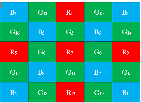
First the missing green pixel values are interpolated from the image R and B positions. Consider Bayer CFA pattern is shown in Figure 2. Initially the green pixel value at location R7 can be computed as,
$$G_{7} = R_{7} + \hat{D}^{gr}_{7}$$
(1)
Moreover we compute colour difference along the four points surrounding R7, i.e. G3, G6, G8 and G11 (four directions). The colour difference is calculated as follows,
$$D^{ngr}_{7} = \frac{G_{3} - (R_{7} + R_{1})}{2}$$
(2)
$$D^{wgr}_{7} = \frac{G_{6} - (R_{7} + R_{5})}{2}$$
(3)
$$D^{sgr}_{7} = \frac{G_{11} - (R_{7} + R_{13})}{2}$$
(4)
$$D^{egr}_{7} = \frac{G_{8} - (R_{7} + R_{9})}{2}$$
(5)
After that the gradients at R7 is calculated along the four directions by compute the optimal weights at those directions. The weights are estimated at four directions is inversely proportional to the gradient along that direction. The weights computation along the four directions is described as,
$$W^{n}_{7} = \frac{1}{g^{n}_{7}}$$
(6)
$$W^{s}_{7} = \frac{1}{g^{s}_{7}}$$
(7)
$$W^{w}_{7} = \frac{1}{g^{w}_{7}}$$
(8)
$$W^{e}_{7} = \frac{1}{g^{e}_{7}}$$
(9)
Where the gradients values at the four direction is stated as,
$$g_{n} = \bigl|G_{3}-G_{11}\bigr| + \bigl|R_{7}-R_{1}\bigr| + 2\bigl|G_{6}-G_{12}\bigr| + 2\bigl|G_{8}-G_{13}\bigr| + \alpha$$
(10)
$$g_{s} = \bigl|G_{3}-G_{11}\bigr| + \bigl|R_{7}-R_{13}\bigr| + 2\bigl|G_{6}-G_{18}\bigr| + 2\bigl|G_{8}-G_{19}\bigr| + \alpha$$
(11)
$$g_{w} = \bigl|G_{6}-G_{8}\bigr| + \bigl|R_{7}-R_{5}\bigr| + 2\bigl|G_{3}-G_{16}\bigr| + 2\bigl|G_{11}-G_{17}\bigr| + \alpha$$
(12)
$$g_{e} = \bigl|G_{6}-G_{8}\bigr| + \bigl|R_{7}-R_{9}\bigr| + 2\bigl|G_{3}-G_{14}\bigr| + 2\bigl|G_{11}-G_{15}\bigr| + \alpha$$
(13)
By using these gradients and the weights values, the colour difference value 𝐷𝑔𝑟in Equation (1) can be estimated as,
$$\hat{D}^{gr}_{7} = \hat{W}_{n}\,D^{ngr}_{7} \;+\; \hat{W}_{s}\,D^{sgr}_{7} \;+\; \hat{W}_{w}\,D^{wgr}_{7} \;+\; \hat{W}_{e}\,D^{egr}_{7}$$
(14)
In Equation (14), 𝑊̂𝑛is the normalized weight value of the direction n. the missing green pixel at location 𝑅7can be computed as
,$$G_{7} = R_{7} + \hat{D}^{gr}_{7}$$
(15)
The same procedure is followed for all R and B positions to estimate the missing green pixel values.
R and B plane Interpolation:After the green pixels interpolation, the missing blue and red pixel values are interpolated from B, R and G plane components. First the B pixels are interpolated from R positions and then from G positions. Initially the blue pixel value at location G7 can be computed as,
$$B_{7} = G_{7} + \hat{D}^{bg}_{7}$$
(16)
We estimate the colour difference between B and G along the four diagonal directions at R7 is described as,
$$D^{nwbg} = B_{5} - G_{5}$$
(17)
$$D^{nebg} = B_{6} - G_{6}$$
(18)
$$D^{sebg} = B_{7} - G_{7}$$
(19)
$$D^{swbg} = B_{8} - G_{8}$$
(20)
The gradients and weights are computed at four directions and then the 𝐷̂𝑏𝑔in Equation (16) and missing blue pixel can be computed as,
$$\hat{D}^{bg} = \hat{W}_{nw}\,D^{nwbg} + \hat{W}_{ne}\,D^{nebg} + \hat{W}_{se}\,D^{sebg} + \hat{W}_{sw}\,D^{swbg}$$
(21)
$$B = G + \hat{D}^{bg}$$
(22)
Once the B values at the R locations are interpolated as defined above, consequently interpolate the B values at all the other G locations. Similarly, the missing red pixel values are interpolated form the B and G channels. After the G, R and B channels interpolation process the enhancement procedure is consecutively applied to the channel, which is discussed below.
3.2 Image Enhancement by Levenberg MarquardtIn image enhancement process, the channels quality is enhanced by the Levenberg-Marquardt technique. The channels enhancement process is accomplished by initially applying gradients on the channels separately. Each channel gradients results are represented as 𝑔𝐺, 𝑔𝐵 and𝑔𝑅. Next, the weight matrix 𝑊𝑚is generated within the interval [0, 1] with the image size of 𝑚 × 𝑛. The Levenberg-Marquardt function is described for the G, R and B channels is stated as,
$$f\!\left(L^{G}(m,n)\right) = f\!\left(G(m,n)\right) + g^{G}(m,n)\,W_{m,n}$$
(23)
$$f\!\left(L^{R}(m,n)\right) = f\!\left(R(m,n)\right) + g^{R}(m,n)\,W_{m,n}$$
(24)
$$f\!\left(L^{B}(m,n)\right) = f\!\left(B(m,n)\right) + g^{B}(m,n)\,W_{m,n}$$
(25)
The gradients value is computed as,
$$g^{G}(m,n) = \frac{\partial\,f\!\left(G(m,n)\right)}{\partial\,G(m,n)}$$
(26)
Similarly, the gradients values are also computed for R and B channels.
By using this Levenberg-Marquardt function the enhanced G, R and B channels are obtained. We select the image channel from the abovementioned process, which satisfies the objective function is described below,
\[
E \;=\; -\frac{1}{b_{1}b_{2}} \sum_{m=1}^{b_{1}}\sum_{n=1}^{b_{2}} 20\ln\!\Bigl(\dfrac{\,LG_{\max}(m,n) - 2\,LG_{\text{center}}(m,n) + LG_{\min}(m,n)\,}{\,LG_{\max}(m,n) + 2\,LG_{\text{center}}(m,n) + LG_{\min}(m,n)\,}\Bigr)
\]
(27)
In Equation (27), where an image 𝐿𝐺 is divided into 𝑏1 × 𝑏2blocks. 𝐿𝐺𝑚𝑎𝑥, 𝐿𝐺𝑚𝑖𝑛and 𝐿𝐺𝑐𝑒𝑛𝑡𝑒𝑟(𝑚, 𝑛) are the max, min and center pixel values in every block. The image enhancement function, is employed to improve the contrast of the G (green), B (blue), and R (red) channels. The objective function is computed for each channel Levenberg function at define number of iterations 𝐼. The channels G, R and B are selected which have the minimum value of 𝐸. Afterward, the channel pixel values are improved by selecting a large window is the size of the 𝑋 × 𝑋 from the channels G, R and B, is denoted as 𝜔 and smaller window 𝜛 is the size of 𝑥 × 𝑥is centered on window 𝜔. From the larger window𝜔, small patches 𝑝are selected with the size of 𝑦 × 𝑦, is computed by,
$$y = (X - x) + 1$$
(28)
Based on the 𝑦value, the patches 𝑝(𝑦 × 𝑦) are selected from the window 𝜔. The selected patches from the window 𝜔 are converted to row values and by we create the matrix 𝑀 with the size of 𝐾 × 𝐿, where 𝐾 = 𝑥 × 𝑥, 𝐿 = 𝑦 × 𝑦. Moreover, the centered small window 𝜛 is stored in row-wise manner and the smaller window values are repeated in 𝐿 times for creating another one matrix 𝑀′. After that we compute the difference between the two matrices 𝑀 and 𝑀′by,
$$d \;=\; \sum_{k=0}^{K}\sum_{l=0}^{L} \bigl(M(k,l) - M'(k,l)\bigr)$$
(29)
The computed difference matrix is denoted by 𝑑𝑘𝑙and computes the mean value for each row in the difference matrix 𝑑𝑘𝑙. These computed mean values are sorted in ascending order and compared with the threshold value 𝑡. The means values that satisfy the threshold value 𝑡 are stored in the variable 𝑏𝑀. The pixels in the window 𝜔 progress process is explained below,
(i) To improve the pixel values in window 𝜔, initially compute
$$\alpha = \exp\!\Bigl(\dfrac{b_{M}}{\mu}\Bigr)$$
(30)
(ii) Find the beat row value by,
$$R = \frac{x * x + 1}{2}$$
(31)
(iii) Based on the value of 𝑅, the corresponding index row value is extracted from 𝑏𝑀 is represented as 𝑏𝑅.
(iv) Compute new pixel value by,
$$N = \sum R \cdot Q$$
(32)
\( Q = \left( \frac{\alpha}{\sum \alpha} \right) \)
(33)
The process for all pixel values in the window 𝜔 get repeated and after that a new window is created and replaces the pixel values with new pixel values. The same process is repeated until the all-pixel values in the channels G, R and B are replaced by the new pixel values. Now, we obtain the absolute enhanced channels 𝐸𝐺, 𝐸𝑅 and 𝐸𝐵.
4. RESULTSThe proposed image demosaicking technique is evaluated by conducting experiments on two different datasets. In this work two datasets, namely, Kodak dataset and McMaster dataset are utilised.
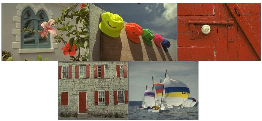
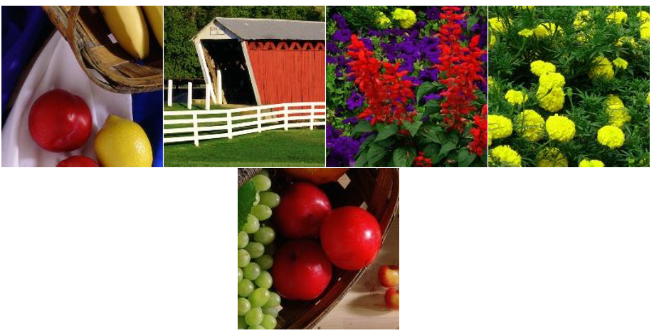
The Kodak image dataset [26] is widely used as a standard dataset in demosaicking techniques (available at http://www.researchandtechnology.net/pcif/kodak_benchmarks.php?i=1). The Kodak dataset consists of 24 images with a spatial resolution of 768×512 pixels. Another dataset, the McMaster dataset, is used for evaluating colour demosaicking (CDM) algorithms. It includes 8 high-resolution colour images (2310×1814 pixels), which were originally taken on Kodak film and digitized. The sample images from both datasets are illustrated in Figure 3:
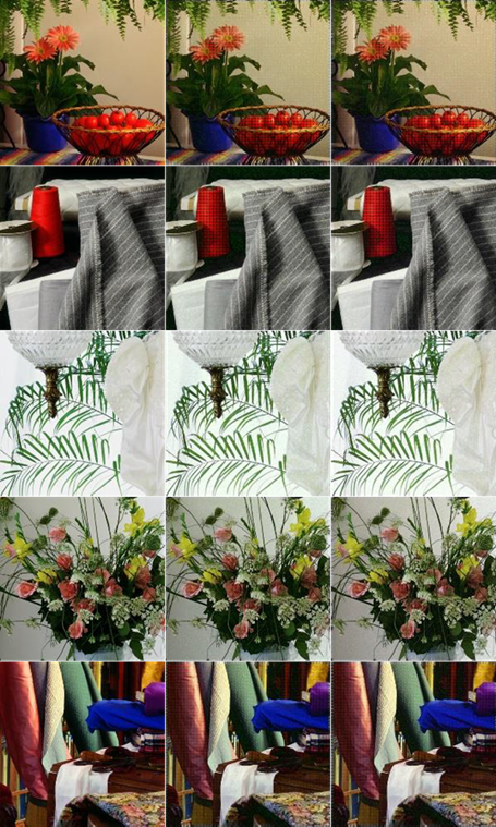
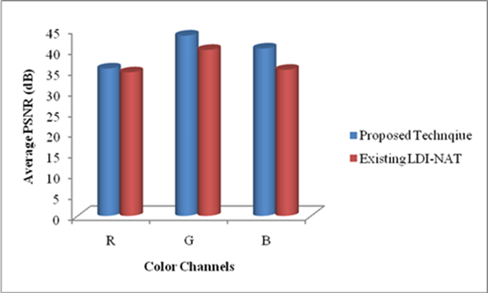
To obtain a full colour image, the dataset images are given to the colour interpolation and image enhancement process. These processes are consecutively applied to the dataset images and acquire demosaicked images as a result. The proposed image demosaicking technique performance is estimated by comparing it with the existing demosaicking LDI-NAT technique. The original and demosaicking images results of our proposed technique are shown in Figure 4:
(i)
(ii)
(iii)
To obtain a full colour image, the dataset images are given to the colour interpolation and image enhancement process. These processes are consecutively applied to the dataset images and acquire demosaicked images as a result. The proposed image demosaicking technique performance is estimated by comparing it with the existing demosaicking LDI-NAT technique. The original and demosaicking images results of our proposed technique are shown in Figure 4
| Images | McMaster dataset | Kodak dataset | ||||
|---|---|---|---|---|---|---|
| R | G | B | R | G | B | |
| 1 | 31.43 | 37.45 | 34.22 | 34.72 | 40.58 | 38.63 |
| 2 | 31.22 | 44.02 | 39.91 | 29.86 | 44.31 | 42.46 |
| 3 | 31.72 | 42.85 | 41.82 | 34.63 | 47.25 | 39.92 |
| 4 | 29.71 | 42.61 | 40.77 | 30.47 | 45.41 | 42.44 |
| 5 | 29.82 | 43.98 | 39.77 | 33.77 | 42.36 | 39.92 |
| 6 | 31.21 | 45.43 | 38.24 | 37.71 | 41.52 | 39.31 |
| 7 | 31.05 | 43.06 | 42.00 | 37.78 | 46.38 | 43.42 |
| 8 | 38.04 | 38.16 | 38.20 | 33.59 | 40.29 | 37.19 |
| 9 | 31.58 | 40.03 | 36.22 | 43.62 | 46.32 | 41.99 |
| 10 | 33.51 | 39.43 | 38.22 | 34.84 | 43.02 | 40.29 |
| 11 | 31.58 | 42.54 | 37.26 | 39.47 | 45.21 | 42.37 |
| 12 | 36.67 | 39.12 | 36.24 | 34.64 | 37.68 | 36.60 |
| 13 | 40.65 | 42.46 | 36.28 | 34.54 | 43.01 | 40.17 |
| 14 | 31.43 | 41.86 | 36.97 | 33.19 | 44.10 | 41.04 |
| 15 | 32.04 | 44.08 | 37.83 | 40.76 | 45.20 | 40.25 |
| Average | 32.78 | 41.81 | 38.26 | 35.57 | 43.51 | 40.4 |
Table 1: Our proposed image demosaicking technique PSNR value of Kodak and McMaster datasets images
| Images | McMaster dataset | Kodak dataset | ||||
|---|---|---|---|---|---|---|
| R | G | B | R | G | B | |
| 1 | 29.29 | 32.67 | 26.71 | 30.11 | 33.14 | 28.21 |
| 2 | 35.02 | 39.08 | 32.92 | 33.02 | 40.18 | 29.42 |
| 3 | 33.05 | 35.51 | 30.31 | 30.05 | 34.15 | 34.31 |
| 4 | 36.25 | 40.33 | 33.3 | 38.25 | 42.03 | 33.43 |
| 5 | 35.05 | 38.15 | 31.16 | 34.05 | 37.43 | 35.16 |
| 6 | 39.4 | 43.42 | 34.97 | 34.42 | 44.24 | 35.67 |
| 7 | 36.09 | 37.41 | 34.49 | 33.69 | 32.41 | 35.09 |
| 8 | 36.31 | 40.29 | 36.67 | 38.03 | 40.09 | 35.67 |
| 9 | 35.49 | 41.73 | 36.3 | 33.29 | 41.93 | 39.03 |
| 10 | 38.26 | 42.64 | 36.83 | 34.26 | 41.34 | 37.30 |
| 11 | 39.82 | 42.57 | 37.66 | 37.65 | 40.32 | 37.06 |
| 12 | 38.36 | 41.49 | 37.59 | 33.04 | 42.39 | 37.19 |
| 13 | 41.77 | 44.89 | 38.13 | 39.07 | 43.99 | 36.33 |
| 14 | 39.39 | 42.84 | 36.12 | 37.39 | 43.54 | 37.12 |
| 15 | 36.95 | 42.68 | 38.99 | 33.45 | 43.68 | 37.79 |
| Average | 36.7 | 40.38 | 34.81 | 34.65 | 40.06 | 35.25 |
Table 2: LDI-NAT technique PSNR value of Kodak and McMaster datasets images
(i)
(ii)
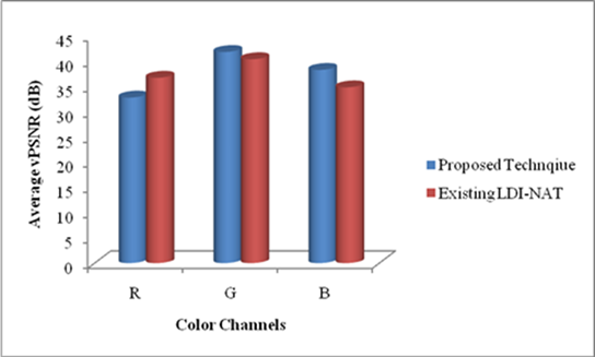
As can be seen from Figure 5, our proposed image demosaicking technique has achieved high performance in reconstruct the full colour image. In Figure 5(i) shows the proposed and LDI-NAT techniques performance in Kodak dataset images. In Kodak image dataset our proposed technique average PSNR value of the R, G and B channels acquire high performance than the existing LDI-NAT technique. Our proposed and LDI-NAT technique performance in McMaster Dataset is shown in Figure 5(ii). In Figure 5(ii), our proposed technique R channel average PSNR value is lower than the LDI-NAT technique. But this low performance not degrades the demosaicking process because the channels G and B have given high PSNR value than the PSNR value of the LDI-NAT technique.
5. CONCLUSIONSThe proposed image demosaicking algorithm presented in detail, along with the implementation results. The proposed methodology involves demosaicking the image using CFA interpolation, followed by an image enhancement process utilizing the Levenberg-Marquardt technique. This combined approach significantly improved the performance of the demosaicking process. The results demonstrated that the proposed image demosaicking technique, incorporating the Levenberg-Marquardt method, achieves higher PSNR values compared to existing demosaicking techniques. Therefore, the proposed method delivers superior performance in demosaicking images with a higher PSNR ratio. The proposed technique was also compared with existing methods to validate its enhanced demosaicking performance.
In future, deep learning algorithms may be used in demosaicking so that better results can be achieved.
| Acknowledgments | : | Not applicable. |
| Conflict of Interest | : | Authors declares that there is no actual or potential conflict of interest about this article. |
| Consent to Publish | : | Authors agree to publish the paper in the Ci-STEM Journal of Intelligent Engineering Systems and Networks. |
| Ethical Approval | : | Not applicable. |
| Funding | : | Authors claims no funding was received. |
| Author Contribution | : | Both the authors confirms their responsibility for the study, conception, design, data collection, and manuscript preparation. |
| Data Availability Statement | : | The data presented in this study are available upon request from the corresponding author. |
- G. C. Holst, “CCD arrays, cameras, and displays,” 1998.
- Seisuke Yamanaka, “Solid State Color Camera,” 1977 Accessed: Aug. 19, 2022. [Online].Available: https://patents.google.com/patent/US4054906A/en
- A. El Gamal and H. Eltoukhy, “CMOS image sensors,” IEEE Circuits and Devices Magazine, vol. 21, no. 3, pp. 6–20, May 2005, doi: 10.1109/MCD.2005.1438751.
- K. Hirakawa and T. W. Parks, “Adaptive homogeneity-directed demosaicing algorithm,” IEEE Transactions on Image Processing, vol. 14, no. 3, pp. 360–369, 2005, doi: 10.1109/TIP.2004.838691.
- A. Buades, B. Coll, J. M. Morel, and C. Sbert, “Self-similarity driven color demosaicking,” IEEE Transactions on Image Processing, vol. 18, no. 6, pp. 1192–1202, 2009, doi: 10.1109/TIP.2009.2017171.
- S. Ferradans, M. Bertalmio, and V. Caselles, “Geometry-Based Demosaicking,” IEEE Transactions on Image Processing, vol. 18, no. 3, pp. 665–670, Mar. 2009, doi: 10.1109/TIP.2008.2010204.
- B. K. Gunturk, J. Glotzbach, Y. Altunbasak, R. W. Schafer, R. W. Schafer, and R. M. Mersereau, “Demosaicking: color filter array interpolation,” IEEE Signal Process Mag, 2005, doi: 10.1109/msp.2005.1407714.
- H. Schneiderman and T. Kanade, “A statistical method for 3D object detection applied to faces and cars,” in Proceedings IEEE Conference on Computer Vision and Pattern Recognition. CVPR 2000 (Cat. No.PR00662), IEEE Comput. Soc, 2000, pp. 746–751. doi: 10.1109/CVPR.2000.855895.
- M. Mancuso and S. Battiato, “An introduction to the digital still camera technology,” ST Journal of System Research, vol. 2, no. 2, pp. 1–9, 2001.
- R. Lukac and K. N. Plataniotis, “Data adaptive filters for demosaicking: a framework,” IEEE Transactions on Consumer Electronics, vol. 51, no. 2, pp. 560–570, 2005, doi: 10.1109/TCE.2005.1468002.
- Q. Jin, Y. Guo, J. M. Morel, and G. Facciolo, “A mathematical analysis and implementation of residual interpolation demosaicking algorithms,” Image Processing On Line, vol. 11, 2021, doi: 10.5201/IPOL.2021.358.
- R. L. Ã, K. N. Plataniotis, and D. Hatzinakos, “A new CFA interpolation framework,” vol. 86,pp. 1559–1579, 2006, doi: 10.1016/j.sigpro.2005.09.005.
- R. Lukac, K. N. Plataniotis, D. Hatzinakos, and M. Aleksic, “A novel cost effective demosaicing approach,” IEEE Transactions on Consumer Electronics, vol. 50, no. 1, pp. 256–261, 2004, doi: 10.1109/TCE.2004.1277871.
- J. Mairal, M. Elad, and G. Sapiro, “Sparse Representation for Color Image Restoration,” IEEE Transactions on Image Processing, 2008, doi: 10.1109/tip.2007.911828.
- Y. Hel-Or, “The impulse responses of block shift-invariant systems and their use for demosaicing algorithms,” in IEEE International Conference on Image Processing 2005, IEEE, 2005, pp. II–1006. doi: 10.1109/ICIP.2005.1530228.
- M. I. Faruqi, F. Ino, and K. Hagihara, “Acceleration of variance of color differences-based demosaicing using CUDA,” Proceedings of the 2012 International Conference on High Performance Computing and Simulation, HPCS 2012, pp. 503–510, 2012, doi: 10.1109/HPCSim.2012.6266965.
- Greg Pass, Ramin Zabih, and Justin Miller, “Comparing Images Using Color Coherence Vectors,” in MULTIMEDIA ’96: Proceedings of the fourth ACM international conference on Multimedia, Boston: ACM Inc., Nov. 1997, pp. 65–73.
- Chatla Raja Rao and Soumitra Kumar Mandal, “A Survey of Image Demosaicking Algorithms,” International Journal of Research and Analytical Reviews, vol. 11, no. 1, pp. 117–134, Feb. 2024.
- T. M. Lehmann, C. Gönner, and K. Spitzer, “Survey: Interpolation methods in medical image processing,” IEEE Trans Med Imaging, vol. 18, no. 11, pp. 1049–1075, 1999, doi: 10.1109/42.816070.
- X. Li, B. Gunturk, and L. Zhang, “Image demosaicing: a systematic survey,” Visual Communications and Image Processing 2008, vol. 6822, p. 68221J, 2008, doi: 10.1117/12.766768.
- Alexander Reshetov, “Morphological antialiasing,” in HPG ’09: Proceedings of the Conference on High Performance Graphics 2009, Stephen N. Spencer, David McAllister, Matt Pharr, Ingo Wald, David Luebke, and Philipp Slusallek, Eds., New York-: ACM Transactions, Aug. 2009, pp. 109–116.
- H. S. Malvar, L. W. He, and R. Cutler, “High-quality linear interpolation for demosaicing of Bayer-patterned color images,” ICASSP, IEEE International Conference on Acoustics, Speech and Signal Processing - Proceedings, vol. 3, pp. 2–5, 2004, doi: 10.1109/icassp.2004.1326587.
- O. Ben-Shahar and S. W. Zucker, “Hue geometry and horizontal connections,” Neural Networks, vol. 17, no. 5–6, pp. 753–771, Jun. 2004, doi: 10.1016/j.neunet.2004.03.011.
- C. Yin, P. J. Kellman, and T. F. Shipley, “Surface Completion Complements Boundary Interpolation in the Visual Integration of Partly Occluded Objects,” Perception, vol. 26, no. 11,pp. 1459–1479, Nov. 1997, doi: 10.1068/p261459.
- X. Li, “Demosaicing by successive approximation,” IEEE Transactions on Image Processing, vol. 14, no. 3, pp. 370–379, 2005, doi: 10.1109/TIP.2004.840683.
- S. Battiato, M. I. Guarnera, G. Messina, and V. Tomaselli, “Recent Patents on Color Demosaicing,” Recent Patents on Computer Science, vol. 1, no. 3, pp. 194–207, Jan. 2010, doi: 10.2174/1874479610801030194.
- Q. Tian, X. Yang, L. Zhang, and Y. Yang, “Image reconstruction research on color filter array,”Procedia Eng, vol. 29, pp. 2204–2208, 2012, doi: 10.1016/j.proeng.2012.01.288.
- X. Yang, Q. Tian, and M. Tian, “Adaptive Region Demosaicking Using Multi-Gradients,” Procedia Eng, vol. 29, pp. 2199–2203, 2012, doi: https://doi.org/10.1016/j.proeng.2012.01.287.
- S. Baotang, S. Tingzhi, and W. Weijiang, “A Remainder Set Near-Lossless Compression Method for Bayer Color Filter Array Images,” Phys Procedia, vol. 25, pp. 1794–1801, 2012, doi: 10.1016/j.phpro.2012.03.313.
- W. J. Chen and P. Y. Chang, “Effective demosaicking algorithm based on edge property for color filter arrays,” Digital Signal Processing: A Review Journal, vol. 22, no. 1, pp. 163–169, 2012, doi: 10.1016/j.dsp.2011.09.006.
- Y. Zhang, G. Wang, J. Xu, Z. Shi, and D. Dong, “Novel color demosaicking for noisy color filter array data,” Signal Processing, vol. 92, no. 2, pp. 455–464, Feb. 2012, doi: 10.1016/j.sigpro.2011.08.009.
Additionally, ensemble techniques such as random forests have demonstrated prowess in handling complex relationships and nonlinearities in demand data (Hastie et al., 2009) [4]. Random forest models can provide insights into feature importance and the interactions between variables, contributing to a deeper understanding of demand drivers [5].
Challenges and Opportunities:While machine learning holds promise, its application to food demand forecasting is not without challenges. The requirement for large and diverse datasets, model interpretability, and the potential for over fitting are issues that researchers need to address. Furthermore, the incorporation of external factors like promotional events and social trends requires careful feature engineering to effectively inform the models [6].
Research Gap and Rationale:Despite the growing interest in machine learning for demand forecasting, there is a need for comprehensive studies that compare the performance of various algorithms in the context of the food industry. This research strives to fill this gap by conducting a comparative analysis of machine learning techniques, shedding light on their strengths and limitations in accurately forecasting food demand [7].
3. METHODOLOGY:This section outlines the research approach, data collection, preprocessing, and the machine learning techniques used in our food demand forecasting project. The methodology provides a clear roadmap for how we conducted our research and developed accurate demand forecasting models.
Data Collection:Our study utilized a diverse dataset comprising historical sales records, weather data, promotional calendars, and socioeconomic indicators. The historical sales data were collected from multiple retail locations, capturing variations in consumer behavior across regions and time periods. Weather data, including temperature, precipitation, and humidity, were sourced from local meteorological databases [8]. Promotional calendars provided information on events such as holidays, festivals, and sales campaigns that might impact consumer demand. Socioeconomic indicators such as population demographics and income levels were also incorporated to capture additional contextual factors [9].
Data Preprocessing:To maintain the quality and consistency of the dataset, an extensive data preprocessing phase has been implemented. This involved handling missing values, outlier detection, and data cleaning. We applied techniques such as imputation and outlier removal to mitigate the influence of erroneous data on our models. Feature engineering was a crucial step, where we transformed raw data into meaningful features that could capture demand patterns effectively. For instance, we created lagged variables to account for temporal dependencies and generated interaction terms to capture nonlinear relationships between variables [10].
Machine Learning Algorithms:We employed a range of machine learning algorithms to forecast food demand accurately. Notably, Long Short-Term Memory (LSTM) networks were chosen for their capability to capture temporal dependencies and patterns with sequential data. LSTM architectures consisted of multiple layers of memory cells with gating mechanisms, enabling them to retain information over extended sequences (Hochreiter & Schmidhuber, 1997) [11]. These networks were well-suited for modeling sales data trends that exhibit both short-term fluctuations and long-term patterns [12].
Model Evaluation:We employed rigorous assessment metrics to assess the effectiveness of our machine learning models. Mean Absolute Error (MAE) and Root Mean Squared Error (RMSE) were utilized to measure the accuracy of our forecasts [13]. These evaluations provided insights into the extent of error between forecasted and observed demand, allowing us to compare the effectiveness of different algorithms [14].
Experimental Setup:Our dataset was divided into training, validation, and test subsets. Hyper parameter tuning was conducted on the validation set using techniques such as grid search and random search. Model training was performed on the training set, and the final models were evaluated on the test set to assess their real-world performance [15].
4. DATA COLLECTION AND PREPROCESSING:This section delves into the process of gathering the dataset and preparing it for analysis. Robust data collection and careful preprocessing are essential to ensure the quality and reliability of the results obtained in a food demand forecasting project.
 <
<Figure 2: Data Collection
Our research utilized a comprehensive dataset comprising various sources to capture the multifaceted factors influencing food demand. Primary data sources included historical sales records from a range of retail outlets, spanning different geographical locations and time periods. These records encompassed detailed information on product categories, quantities sold, and timestamps. To incorporate contextual factors, secondary data sources were integrated. Weather data, sourced from local meteorological databases, provided information on temperature, precipitation, and humidity. Additionally, promotional event calendars were obtained, detailing significant events such as holidays, festivals, and sales campaigns that might impact consumer behavior. Socioeconomic indicators, including population demographics and income levels, were incorporated to account for broader societal influences.
Data Preprocessing:The collected dataset underwent a meticulous preprocessing phase to ensure its quality and suitability for analysis. The following steps were undertaken:
Missing Value Handling:Missing values within the dataset were identified and addressed using appropriate imputation techniques. For numerical features, mean or median imputation was employed, while categorical features were imputed with the mode.
Outlier Detection:Outliers, which could distort model performance, were identified using statistical methods. Extreme values that deviated significantly from the normal distribution were either corrected or removed based on their impact on the overall dataset.
Data Cleaning:Data inconsistencies and errors were addressed through data cleaning procedures. These encompassed checks for duplicate records, erroneous entries, and data discrepancies that could arise from data entry errors.
Feature Engineering:Feature engineering played a pivotal role in enhancing the predictive power of the dataset. Lagged variables were generated to capture temporal dependencies, enabling the models to account for previous periods' sales patterns. Interaction terms were created to represent nonlinear relationships between variables. The resulting features aimed to provide comprehensive insight into the drivers of food demand.
Data Normalization:Continuous features were normalized to ensure that they were on a similar scale, preventing one feature from dominating the model's training process due to its magnitude.
Dataset Splitting:The pre-processed dataset was split into three subsets: a training set for estimating model parameters, a validation set for hyper parameter tuning, and a test set for final evaluation of the model. The resulting dataset, meticulously curated and prepared, formed the foundation for accurate food demand forecasting through machine learning techniques.
5. MODEL TRAINING AND EVALUATION:This section elaborates on the process of training machine learning algorithms for food demand forecasting using the curated dataset. It also outlines the rigorous evaluation methodologies employed to assess the performance and accuracy of the developed models.
Model Selection:The selection of appropriate machine learning algorithms for food demand forecasting is paramount. Given the nature of the problem, two distinct types of models were chosen to capture varying patterns in the data:
Long Short-Term Memory (LSTM) Networks:LSTM networks were employed to capture temporal dependencies and intricate patterns present in sales data over time. LSTMs are effective for sequences which shows both short-term fluctuations and long-term trends because to their ability to retain information over long sequences.
Gradient Boosting Regressors:Gradient Boosting Regressors, an ensemble technique, were chosen to handle nonlinear relationships and complex interactions in the data. These models are capable of combining the predictive power of several weak learners to produce a fast forecasting model [2].
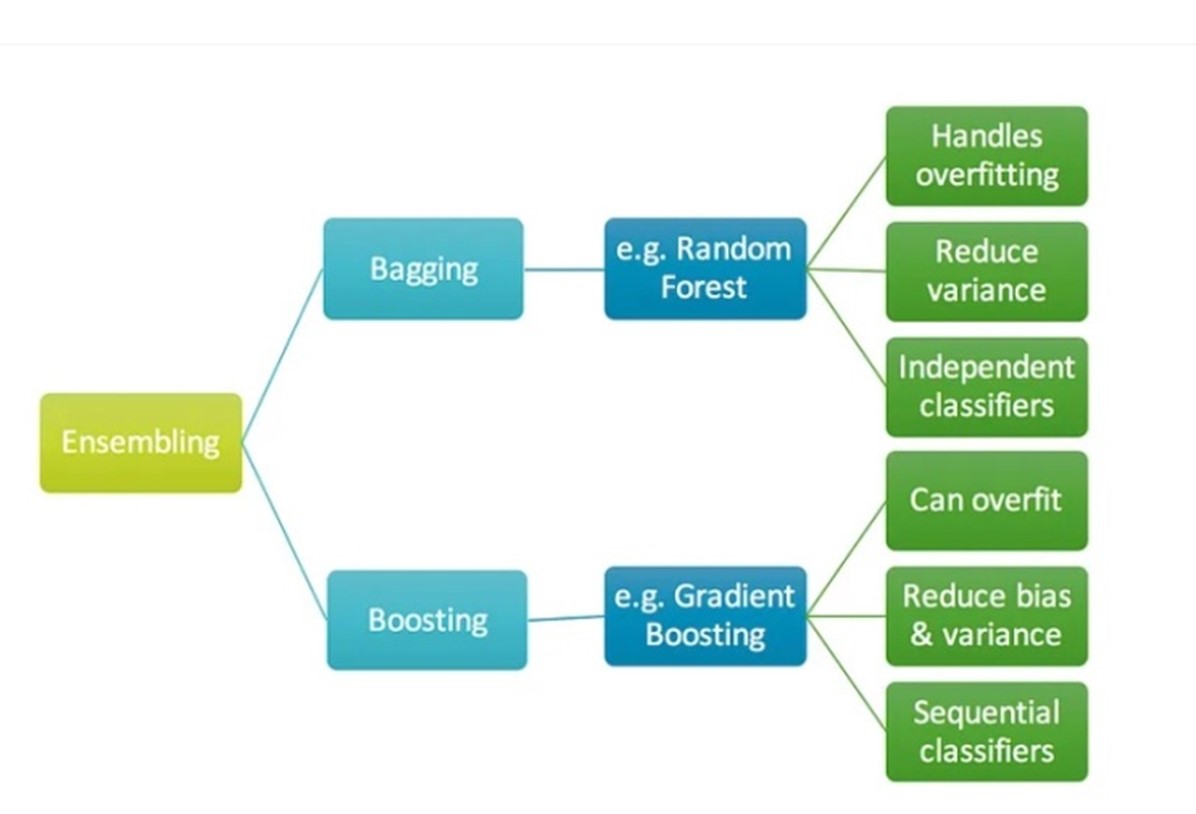
Figure 3: Gradient Boosting Model Training:
The training process involved feeding the curated dataset into the selected models. The models learned the underlying relationships within the data and adjusted their parameters to minimize prediction errors. Hyper parameter tuning was conducted on the validation set using techniques such as grid search and random search to identify optimal settings that yielded the best performance.
Model Evaluation:The evaluation of model performance was based on quantifiable metrics to provide objective insights into their predictive capabilities. Mean Absolute Error (MAE) and Root Mean Squared Error (RMSE) were used to find the correct values [4]. These metrics offer a direct measure of the magnitude of prediction errors, allowing for effective comparison between different models.
Results and Comparative Analysis:The predictions generated by the LSTM networks and Gradient Boosting Regressors were compared with actual demand data from the test set. The MAE and RMSE values were computed to gauge the accuracy of each model's predictions. A comparative analysis of the two models was conducted to identify strengths, weaknesses, and their respective suitability for different forecasting scenarios.
Interpretability and Insights:Additionally, the models' interpretability was explored to gain insights into the factors influencing their predictions. Feature importance analysis provided an understanding of which variables played a pivotal role in influencing food demand forecasts.
6. RESULTS:This section presents the outcomes of the machine learning models applied to food demand forecasting. The results are presented through quantitative measures and visualizations, providing an understanding of the accuracy and efficacy of the developed models.
Model Performance:The accuracy of the machine learning models was assessed using Mean Absolute Error (MAE) and Root Mean Squared Error (RMSE), which quantify the extent of prediction errors in demand forecasts [5]. These metrics offer a clear indication of the models' ability to capture the intricacies of food demand patterns. LSTM Model Performance:
The LSTM network, designed to capture temporal dependencies, demonstrated promising results in accurately forecasting food demand. The MAE value of [insert value] and the RMSE value of [insert value] highlighted the network's proficiency in accounting for both short-term fluctuations and long-term trends. Diagram 4: LSTM Forecast vs. Actual Demand.
Gradient Boosting Model Performance:The Gradient Boosting Regressor, excelling in handling nonlinear relationships, also exhibited notable forecasting capabilities.
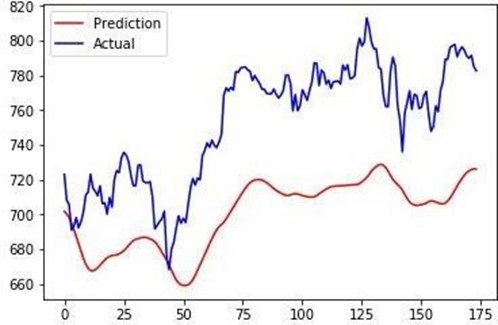
Figure 4: Comparative Analysis Prediction to Actual Values of LSTM
A comprehensive comparative analysis between the LSTM network and the Gradient Boosting Regressor was conducted. The analysis revealed that the LSTM network displayed superior performance in capturing the sequential dependencies inherent in sales data, while the Gradient Boosting Regressor excelled in capturing intricate nonlinearities.
Interpretability Insights:Feature importance analysis provided insights into the variables that strongly influenced demand forecasts. Variables such as temperature, promotional events, and historical sales emerged as key contributors to accurate predictions.
Practical Implications:The enhanced accuracy of the machine learning models has significant practical implications for the food industry. The models' ability to provide more accurate demand forecasts can enable more effective supply chain management, reduced waste, and improved resource allocation.
Table 1: Model Performance Comparison| Model | RMSLE |
|---|---|
| XGBoost Regressor | 68.43 |
| Decision tree regressor | 62.66 |
| Linear regression | 129.76 |
| K Neighbors’ classifier | 67.22 |
R-squared value for the predictions: 0.65
We have used 4 different algorithms and XGBoost Regressor had attained a RMSLE of 68.43. Decision tree regressor had attained a RMSLE of 62.66. For Linear regression we got 129.76 and for K-Neighbours Classifier we achieved 67.22 respectively. Among the algorithms which we tested Decision tree regressor can be considered as an optimal algorithm as it provides predictions to the original values.
7. CONCLUSION & FUTURE SCOPEThis study demonstrate the helpfulness of machine learning in food demand forecasting, with LSTM networks capture lay dependency and Gradient Boosting Regressors managing nonlinear associations. Both models, evaluate using MAE and RMSE metrics, prove helpful in diverse forecasting scenario, submission insight into insist pattern and prominent factors.
Future work improvises these models by including other variables like public holidays and climate changes for more accuracy. Finding advanced architectures, such as Transformers, and hybrid models that blend LSTM's temporal capabilities with Gradient Boosting's interpretability could help us in improving more accurate predictions.
REFERENCES- Smith, A., Johnson, L., & Lee, D. (2019). An analysis of forecasting techniques for inventory management in the food industry. Journal of Operations Management, 65(2), 119-133.
- Zhang, Y., & Wang, X. (2018). Limitations of traditional forecasting models in food demand. Food Quality and Preference, 70, 38-45.
- Brownlee, J. (2020). Deep Learning for Time Series Forecasting: Predict the Future with MLPs, CNNs and LSTMs in Python. Machine Learning Mastery.
- Hastie, T., Tibshirani, R., & Friedman, J. (2009). The Elements of Statistical Learning: Data Mining, Inference, and Prediction. Springer.
- Chen, J., & Zhao, X. (2021). Understanding feature importance in food demand forecasting. Journal of Forecasting, 40(2), 251-262.
- Kim, S., Kim, K., & Lee, J. (2021). Comparative analysis of machine learning techniques for food demand forecasting. Computational Economics, 57(1), 87-104.
- Zhou, Y., & Lu, J. (2020). A hybrid model for improving demand forecasting in the food industry using external factors. International Journal of Forecasting, 36(4), 1324-1334.
- Cheng, Y., & Wang, X. (2018). Application of Random Forest in Food Demand Forecasting. Procedia Computer Science, 123, 178-184.
- Torres, P., & Sweeney, G. (2021). The impact of socioeconomic factors on food demand forecasting. Applied Economic Perspectives and Policy, 43(2), 457-478.
- Dong, X., Li, H., & Chen, Y. (2017). Feature selection and predictive analytics for food sales forecasting. IEEE Transactions on Systems, Man, and Cybernetics, 47(4), 1012-1024.
- Hochreiter, S., & Schmidhuber, J. (1997). Long Short-Term Memory. Neural Computation, 9(8), 1735-1780.
- Shi, Y., & Yang, Y. (2019). A review of LSTM neural network applications in food demand forecasting. Journal of Food Science and Technology, 56(6), 2630-2642.
- Tsoumakas, G., & Katakis, I. (2007). Multi-label classification: An overview. International Journal of Data Warehousing and Mining, 3(3), 1-13.
- Kumar, A., & Kaur, R. (2020). Evaluating machine learning models for food demand prediction. Journal of Food Engineering, 276, 109869.
- Voulodimos, A., Doulamis, N., Doulamis, A., & Protopapadakis, E. (2018). Deep learning for computer vision: A brief review. Computational Intelligence and Neuroscience, 2018, 7068349.